Free-Space Fresnel Propagation with abcdLux¤
This tutorial is designed as an introduction to the new abcdLux backend propagators for dLux. This library is still in development but adds a huge amount of flexibility and functionality to dLux's propagation capabilities. It provides full paraxial Fresnel propagation capabilities through the Angular Spectrum Method (ASM) and the Linear Canonical Transform (LCT), allows optical systems to be described and modelled through a series of abcd matrices, provides explicit propagation kernel caching, and provides a more general set of 2-sided Matrix Fourier Transform (MFT) propagators. dLux provided a number of high-level propagator wrappers for these functionalities, however this module is still considered in-development and is subject to change.
This tutorial will cover a basic example showing the free-space ASM propagation, to model realistic out-of-plane optical diffraction.
# Basic imports
import jax.numpy as np
from jax import jit

# dLux imports
import dLux as dl
import dLux.utils as dlu

# Visualisation imports
from tqdm.notebook import tqdm
import matplotlib.pyplot as plt
import matplotlib as mpl

%matplotlib inline
plt.rcParams['image.cmap'] = 'inferno'
plt.rcParams["font.family"] = "serif"
plt.rcParams["image.origin"] = 'lower'
plt.rcParams['figure.dpi'] = 120

# Nan friendly colormapping
inferno = mpl.colormaps["inferno"]
seismic = mpl.colormaps["seismic"]
inferno.set_bad("k", 0.5)
seismic.set_bad("k", 0.5)
Construct our diffraction grating
# Define the grating size
diam = 0.0012  # 1.2 mm diameter
wf_npix = 128
osamp = 8
coords = dlu.pixel_coords(wf_npix * osamp, diam)
cens = np.linspace(-diam / 3, diam / 3, 4)

# Construct the grating
slits = []
for i in range(len(cens)):
    loc = coords - np.array([cens[i], 0.])[:, None, None]
    rect = dlu.rectangle(loc, width=diam / 20, height=diam)
    slits += [rect, rect.T]
grating = np.clip(np.sum(np.array(slits), axis=0), 0, 1)
grating = dlu.downsample(grating, osamp, mean=True)
Build our optical system with a simple ASM free-space propagation, and propagate some optical wavelengths.
# Construct the optical system with the ASM propagator
optics = dl.LayeredOpticalSystem(
    wf_npixels=wf_npix,
    diameter=diam,
    layers=[
        ("aper", dl.TransmissiveLayer(grating, normalise=True)),
        ("asm", dl.ASMPropagator(distance=1.0, spec=dl.PadSpec(pad=20, crop=2))),
    ],
)

# Define the spectral wavelengths and weights
wavels = 1e-9 * np.linspace(380, 780, 30)
weights = np.linspace(1, 0.3, len(wavels))
psf = optics.propagate(wavels, weights=weights, return_wf=True).psf
These cells are just to turn our PSFs into a nice RGB image for display. The RGB conversion function is build from diffractsim and color-matching function table is also taken from the same source.
RGB conversion function
from numpy import loadtxt

def rgb_from_psfs(psfs, wavelength, gamma=True):
    """
    Convert a stack of spectrally weighted PSFs into an RGB image using the same colour
    logic as diffractsim.

    Parameters
    ----------
    psfs : array, shape (nlam, ny, nx)
        Spectrally weighted intensity images per wavelength.
    wavelengths : array, shape (nlam,)
        Wavelengths in meters.
    gamma : bool
        Apply the same sRGB gamma correction as diffractsim.

    Returns
    -------
    rgb : array, shape (ny, nx, 3)
        RGB image in [0, 1].
    """
    psfs = np.asarray(psfs, dtype=float)
    wl = 1e9 * np.asarray(wavelength, dtype=float).reshape(-1)

    if psfs.shape[0] != wl.shape[0]:
        raise ValueError(
            f"psfs.shape[0]={psfs.shape[0]} but len(wavelengths)={len(wl)}"
        )

    # CIE colour matching function
    cmf = loadtxt("cie-cmf.txt")
    wl_cmf = cmf[:, 0]
    xbar_tab = cmf[:, 1]
    ybar_tab = cmf[:, 2]
    zbar_tab = cmf[:, 3]

    # Interpolate CMFs onto your wavelength grid
    xbar = np.interp(wl, wl_cmf, xbar_tab, left=0.0, right=0.0)
    ybar = np.interp(wl, wl_cmf, ybar_tab, left=0.0, right=0.0)
    zbar = np.interp(wl, wl_cmf, zbar_tab, left=0.0, right=0.0)

    # Use this overall scale in spec_to_XYZ
    # If your wavelengths are not uniformly spaced, use local spacing.
    dlam = np.gradient(wl)
    scale = dlam * 0.003975 * 683.002

    # Spectrum -> XYZ
    X = np.sum(psfs * (xbar * scale)[:, None, None], axis=0)
    Y = np.sum(psfs * (ybar * scale)[:, None, None], axis=0)
    Z = np.sum(psfs * (zbar * scale)[:, None, None], axis=0)

    XYZ = np.stack([X, Y, Z], axis=0)  # (3, ny, nx)

    # XYZ -> linear sRGB, same matrix as diffractsim
    T = np.array(
        [
            [3.2406, -1.5372, -0.4986],
            [-0.9689, 1.8758, 0.0415],
            [0.0557, -0.2040, 1.0570],
        ],
        dtype=float,
    )

    rgb = np.tensordot(T, XYZ, axes=([1], [0]))  # (3, ny, nx)

    # "add white" clipping for negative values
    rgb_min = np.amin(rgb, axis=0)
    rgb_max = np.amax(rgb, axis=0)
    scaling = np.where(
        rgb_max > 0.0,
        rgb_max / (rgb_max - rgb_min + 1e-5),
        1.0,
    )
    rgb = np.where(
        rgb_min[None, ...] < 0.0,
        scaling[None, ...] * (rgb - rgb_min[None, ...]),
        rgb,
    )

    if gamma:
        # sRGB gamma
        rgb = np.where(
            rgb <= 0.00304,
            12.92 * rgb,
            1.055 * np.power(np.maximum(rgb, 0.0), 1.0 / 2.4) - 0.055,
        )

        # highlight scaling
        rgb_max = np.amax(rgb, axis=0) + 1e-5
        rgb = np.where(
            rgb_max[None, ...] > 1.0,
            rgb / rgb_max[None, ...],
            rgb,
        )

    rgb = np.moveaxis(rgb, 0, -1)  # (ny, nx, 3)
    rgb = np.clip(rgb, 0.0, 1.0)

    return rgb
Plotting code
rgb = rgb_from_psfs(500 * psf, wavels)

aper_ext = dlu.imshow_extent(1e3 * diam)
psf_ext = dlu.imshow_extent(1e3 * diam * optics.pad / optics.crop)

plt.figure(figsize=(10, 4))
ax = plt.subplot(1, 2, 1)
im = ax.imshow(grating, extent=aper_ext)
ax.set(title="Grating", xlabel="x (mm)", ylabel="y (mm)")
plt.colorbar(im, ax=ax, label="Transmission")

ax = plt.subplot(1, 2, 2)
im = ax.imshow(rgb, extent=psf_ext)
ax.set(title=f"PSF: z={1.0} m", xlabel="x (mm)", ylabel="y (mm)")
plt.tight_layout()
plt.show()
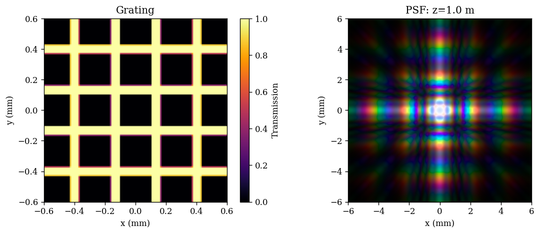
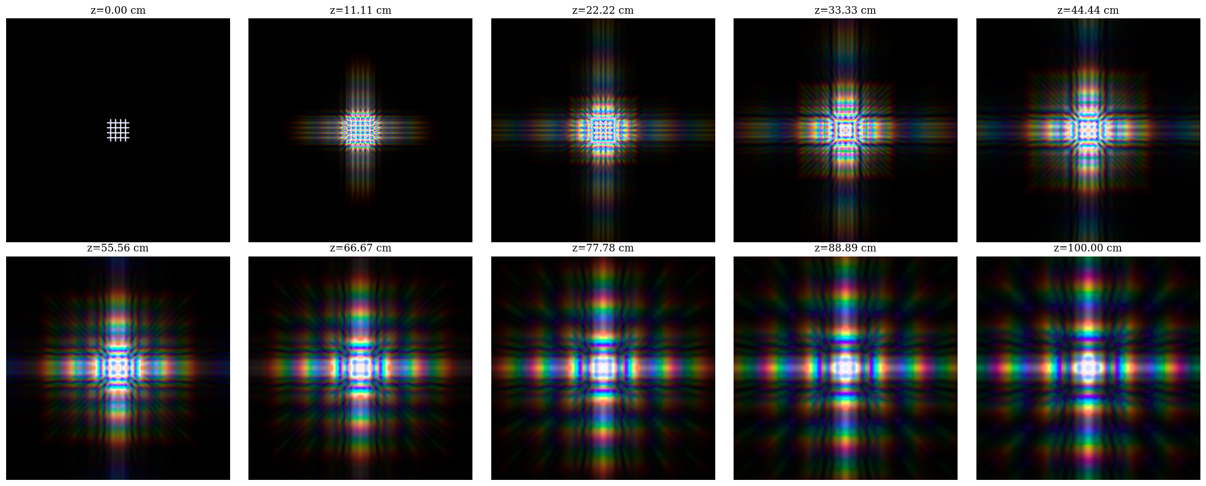
That looks pretty awesome! Now lets use this function to watch the PSF actually evolve as it propagates through free-space, we can just propagate the PSF to a number of different planes and convert each one to RGB for display.
# Build our propagation functions
spectral_fn = lambda wl, optx: optx.propagate(wl, weights=weights, return_wf=True).psf
prop_fn = jit(lambda z, wl: spectral_fn(wl, optics.set("distance", z)))

# Define our propagation distances
zs = np.linspace(0, 1, 10)

# Propagate to each plane and collect the PSFs. Note we do this one distance at a time
# to avoid hitting RAM limits and slowing down from memory swap
psfs = []
for z in tqdm(zs):
    psfs.append(prop_fn(z, wavels).block_until_ready())

# Convert to RGB
rgbs = [rgb_from_psfs(500 * psf, wavels) for psf in psfs]
0%| | 0/10 [00:00<?, ?it/s]
Plotting code
plt.figure(figsize=(20, 8))
for i in range(10):
    plt.subplot(2, 5, i + 1)
    plt.imshow(rgbs[i], extent=psf_ext)
    plt.title(f"z={100*zs[i]:.2f} cm")
    plt.axis("off")
plt.tight_layout()
plt.show()
If you are running this locally, you can save these as a nice video!
Animation code
import matplotlib.pyplot as plt
from matplotlib import animation
from IPython.display import HTML

# Add some start and stop frames to make the animation pause at the ends
rgbs = 10 * [rgbs[0]] + rgbs + 10 * [rgbs[-1]]
plt_zs = 10 * [zs[0]] + list(zs) + 10 * [zs[-1]]

fig, ax = plt.subplots(figsize=(5, 5), dpi=80)

im = ax.imshow(rgbs[0], extent=psf_ext)
title = ax.set_title(f"PSF: z={100 * plt_zs[0]:.2f} cm")
ax.set_xlabel("x (mm)")
ax.set_ylabel("y (mm)")
plt.tight_layout()

def update(i):
    im.set_data(rgbs[i])
    title.set_text(f"PSF: z={100 * plt_zs[i]:.2f} cm")
    return im, title

anim = animation.FuncAnimation(
    fig,
    update,
    frames=len(rgbs),
    interval=200,
    blit=False,
)

plt.close(fig)
HTML(anim.to_jshtml())
# Save the animation
anim.save("psf_animation.mp4", writer="ffmpeg")